Statistical Reliability and Psychological Reliability
Discussion and Programs
Yasuharu Okamoto, 2018, 2022
Discussion
Two types of reliability of a psychological scale of categorical items should be distinguished. One is statistical reliability and the other is psychological reliability. In the case of continuous items, values of statistical reliability and psychological reliability coincide. However, in general, in the case of categorical items, statistical reliability coefficients, among which the coefficient alpha is the most common, overestimate psychological reliability. In the case of categorical items, the two types of reliability are defined on essentially different kinds of models. This difference would be considered to concern the problem of realism in the philosophy of science.
Statistical reliability is based on the
same kind of model as is used for continuous items. That is, an observed value ![]() on categorical item
on categorical item ![]() of person
of person ![]() is represented as the
sum of a true value
is represented as the
sum of a true value ![]() and an error
and an error ![]() , that is,
, that is,
![]()
The true value ![]() of categorical response
of categorical response ![]() is defined as
expectation of
is defined as
expectation of ![]() ,
,
![]()
These formulations (1) and (2) well
correspond to those of classical test theory for continuous items. But, for
categorical items, a response ![]() is assumed to take an
integer value. So, it seems natural to think that the true value of a
categorical item
is assumed to take an
integer value. So, it seems natural to think that the true value of a
categorical item ![]() be also an integer
value. It seems statistical convenience to define the true value as expectation
of the observed value. By defining the true value as expectation of a
categorical variable, statistical argument on reliability can be done as in the
case of continuous items, although the true value may not be integer. The
common coefficient alpha
be also an integer
value. It seems statistical convenience to define the true value as expectation
of the observed value. By defining the true value as expectation of a
categorical variable, statistical argument on reliability can be done as in the
case of continuous items, although the true value may not be integer. The
common coefficient alpha ![]() can be considered to be
calculated based on this framework where the true value is defined
statistically as expectation of categorical variable
can be considered to be
calculated based on this framework where the true value is defined
statistically as expectation of categorical variable ![]() .
.
Researchers who employ this definition of the true value as the statistical expectation seem to deny the true value of the concept to be measured as Platonic one.
On the other hand, psychological
reliability is based on a psychological model, which is called Thurstonian model,
or is known as Samejima�fs model in item response theory
(IRT). According to Thurstonian modeling, categorical response ![]() on item
on item ![]() of person
of person ![]() is generated by
categorizing a latent continuous response
is generated by
categorizing a latent continuous response ![]() on item
on item ![]() of person
of person ![]() (Okamoto,
2017). The latent continuous response
(Okamoto,
2017). The latent continuous response ![]() consists of a true value
consists of a true value
![]() and an error
and an error ![]() , that is,
, that is,
![]()
Strength of the psychological concept of
person ![]() is represented by
is represented by ![]() . For model (3), the true value is defined as that of the
psychological concept to be measured. That is, the true value is not a mere
statistical value, but the real value of the concept.
. For model (3), the true value is defined as that of the
psychological concept to be measured. That is, the true value is not a mere
statistical value, but the real value of the concept.
Godfrey-Smith (2021) says:
I think that scientific theories, when things go well, can in principle and often do in fact tell us about how the world works and what it contains, including some of its deeply hidden structure. (p. 236)
He says more:
I think that phenomenal-realism, metaphysical constructivism, and other standard views that oppose realism are false.(ibid. p.236)
If we adopt Godfrey-Smith�fs view of the realism, we should consider that the statistical definition of real value is false. Analysis of psychological scale must be based on realism of the true value, that is, eq.(3). When factor analysis of categorical items is done with polychoric or tetrachoric correlation coefficients, continuous latent variables are assumed.
Under the model (3), the observed
categorical score ![]() on categorical item
on categorical item ![]() of person
of person ![]() is given by
categorization of
is given by
categorization of ![]() , that is,
, that is,
![]()
where ![]() is a category boundary.
is a category boundary.
A score of a psychological scale of ![]() categorical items of
person
categorical items of
person ![]() is given by the sum
is given by the sum ![]() , where
, where

For the model given by Equations (3) to
(5), relation of a true value ![]() , more specifically
, more specifically ![]() , and the observed scale score
, and the observed scale score ![]() can be represented by
the following regression models:
can be represented by
the following regression models:
![]()
or
![]()
Reliability of the scale, which represents
the strength of relation between the observed score ![]() and the true value
and the true value ![]() , can be given by the coefficient of determination
, can be given by the coefficient of determination ![]() -index, which is given by squared correlation of
-index, which is given by squared correlation of ![]() and
and ![]() , the common value for regression models (6) and (7). This
coefficient of reliability given by
, the common value for regression models (6) and (7). This
coefficient of reliability given by ![]() -index is denoted by
-index is denoted by ![]() (Okamoto
(2016)) or
(Okamoto
(2016)) or ![]() (Okamoto
(2017)), and given by
(Okamoto
(2017)), and given by
![]()
Reliability coefficient ![]() or
or ![]() represents the strength
of relation between an observed score
represents the strength
of relation between an observed score ![]() and the true value
and the true value ![]() of the psychological
concept to measure. The popular coefficient of reliability
of the psychological
concept to measure. The popular coefficient of reliability ![]() , which can be considered to be a coefficient of statistical
reliability, tends to overestimate
, which can be considered to be a coefficient of statistical
reliability, tends to overestimate ![]() or
or ![]() (Okamoto,
2016, 2017).
(Okamoto,
2016, 2017).
Python scripts to estimate ![]() (that is,
(that is, ![]() ) were developed and can be downloaded from this website. Formulae
of the calculation are given in appendix of Okamoto (2017)
and rather complex. However, it should be noted that in general, the following
simpler equation is wrong:
) were developed and can be downloaded from this website. Formulae
of the calculation are given in appendix of Okamoto (2017)
and rather complex. However, it should be noted that in general, the following
simpler equation is wrong:
![]()
where ![]() denotes covariance of
denotes covariance of ![]() and
and ![]() conditional on
conditional on ![]() , and
, and ![]() is a probability density
function of
is a probability density
function of ![]() .
.
The following example shows that Equation (9) is wrong.
Set two variables ![]() and
and ![]() as follows:
as follows:
![]()
![]()
Then, denoting expectations of ![]() and
and ![]() by
by ![]() and
and ![]() , we have
, we have
![]()
Since
![]()
we have
![]()
We also have
![]()
Hence, we have
![]()
On the other hand, denoting expectations of
![]() and
and ![]() conditional on
conditional on ![]() by
by ![]() and
and ![]() , and variables
, and variables ![]() and
and ![]() conditional on
conditional on ![]() by
by ![]() and
and ![]() , we have
, we have
![]()
![]()
![]()
where ![]() denotes expectation
conditional on
denotes expectation
conditional on ![]() .
.
Hence, we have
![]()
where ![]() is a density function of
is a density function of
![]() .
.
Equations (10) and (11) shows that Equation (9) does not hold.
Programs for Estimating the Coefficient of
Reliability of Categorical Items
Python scripts using Stan scripts were developed. The models (3) and (4) give probabilities of categorical responses as follows:
![]()
![]()
![]()
Equation (12) shows that an origin and a unit of the scale are arbitrary. To identify parameter values, some restrictions of parameters are needed (Okamoto, 2017). The following programs were developed with these restrictions for model identification, which produced three Stan scripts corresponding to number of item categories: (A) More than three categories, (B) Three categories, and (C) Two categories (i.e., Binary items). These Stan scripts are essentially the same as those for item response theory (IRT), so the approach in this website may be called sum of item responses theory (SIRT).
The Stan scripts estimate parameter values,
with which coefficient of reliability ![]() is calculated by the
class CalcRhoPreRhoYYP declared in the module CalcRho_cat.py. All the files of
Stan script and Python scripts are archived in a zip file with (a) sample data
file(s), and can be downloaded from this website.
is calculated by the
class CalcRhoPreRhoYYP declared in the module CalcRho_cat.py. All the files of
Stan script and Python scripts are archived in a zip file with (a) sample data
file(s), and can be downloaded from this website.
The programs (scripts) can analyze data with missing values. For details on missing values, see the documents on �gHow to use�h, which can be downloaded from this website.
(A)
Items with more than three categories
The following condition
![]()
is set. The origin and unit are set indirectly by restriction (13). The Stan script for condition (13) is shown below (Listing 1). The Stan script file and Python files are archived in a zip file with sample data files. How to use is explained in a document of a pdf file.
Run the Python main script (Figure 1). The name of input data file will be asked. After typing in the input data file name, an output file name will be required.
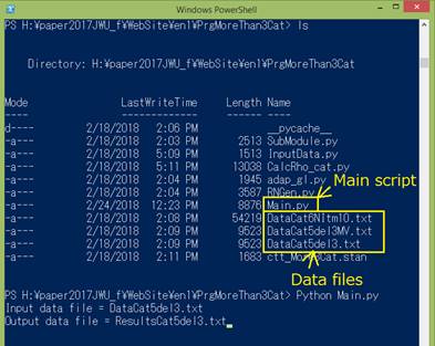
Figure 1
After typing in a output file name, the Stan script will be run, and the point estimates will be calculated. The medians of the distributions are used as the point estimates (Figure 2).
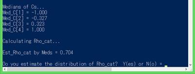
Figure 2
After displaying the point estimate of ![]() , which was calculated using the medians by the class
CalcRhoPreRhoYYP, a message which asks whether estimation of a distribution of
, which was calculated using the medians by the class
CalcRhoPreRhoYYP, a message which asks whether estimation of a distribution of ![]() is needed or not will be
displayed.
is needed or not will be
displayed.
If you do not want to estimate the distribution, type in the character �eN�f. The program will end.
If you type in the character �eY�f, estimation of a distribution of 100 samples, which will be calculated by four parallel processes, each of which displays the current state (Figure 3).
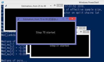
Figure 3
After calculation of the samples, a histogram of the samples will be displayed (Figure 4).
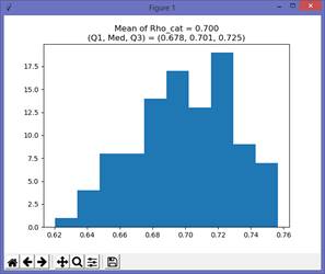
Figure 4
Close this window, the program ends. The results of the calculations are printed out in the output file.
The content of the output file is as follows (Figures 5 to 8):
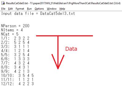
Figure 5
.
.
.
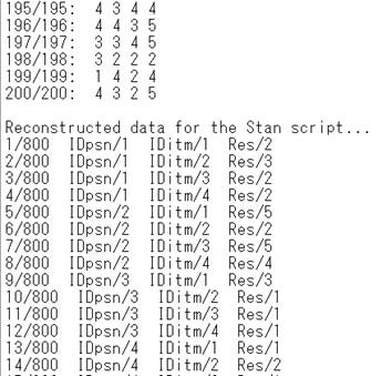
Figure 6
.
.
.
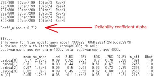
Figure 7
.
.
.
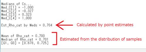
Figure 8
How to use the program is explained in detail with a sample output of the calculation in this document (a pdf file).
The program files and sample data files are archived in this file (a zip file), which can be downloaded.
Listing 1. Stan script for items of more than three categories
// Yasuharu
Okamoto, 2017.07
data {
int <lower = 4>
K;
//
Number of categories > 3
int Npsn;
//
Number of persons
int Nitm;
//
Number of items
int Ntot;
// Number of
data, Ntot <= Nprn * Nitm
int<lower = 1, upper =
Npsn> IDpsn[Ntot]; // Person ID
int<lower = 1, upper =
Nitm> IDitm[Ntot]; // Item ID
int<lower = 1, upper =
K> Res[Ntot];
//
Response-> An integer value between 1 and K
}
parameters {
real<lower = 0.0> Lambda[Nitm];
real
mu[Nitm];
simplex[K - 2] w_c;
real<lower = 0.0> psi[Nitm];
real
F[Npsn];
}
transformed parameters
{
vector[K] p[Ntot];
real C[K - 1];
C[1] = -1.0;
for (k in 2:(K - 1)){
C[k]
= C[k - 1] + w_c[k - 1] * 2.0;
}
for (i in 1:Ntot){
p[i][K] = Phi(((mu[IDitm[i]] + (Lambda[IDitm[i]] * F[IDpsn[i]])) - C[K -
1]) /
psi[IDitm[i]]);
p[i][1] =1.0 -
Phi(((mu[IDitm[i]] + (Lambda[IDitm[i]] * F[IDpsn[i]])) - C[1]) /
psi[IDitm[i]]);
for
(k in 2:(K - 1)){
p[i][k] = Phi(((mu[IDitm[i]] + (Lambda[IDitm[i]] * F[IDpsn[i]])) - C[k -
1]) /
psi[IDitm[i]])
- Phi(((mu[IDitm[i]] + (Lambda[IDitm[i]] * F[IDpsn[i]])) - C[k]) /
psi[IDitm[i]]);
}
}
}
model {
for (i in 1:Npsn)
F[i]
~ normal(0.0, 1.0);
for (i in 1:Ntot)
Res[i] ~ categorical(p[i]);
}
(B)
Items with three
categories
This case is the same as that of more than
three categories, except that only two category boundaries ![]() and
and ![]() are used, so free
category boundary does not exist. The Stan script for items of three categories
is shown in Listing 2. Complete set of the scripts is
archived in this zip file with a sample data
file, and How to use the script are explained in this
document (a pdf file).
are used, so free
category boundary does not exist. The Stan script for items of three categories
is shown in Listing 2. Complete set of the scripts is
archived in this zip file with a sample data
file, and How to use the script are explained in this
document (a pdf file).
The way how to use the scripts is the same as in the case of items of more than three categories, which is explained above.
Run the Python script as follows (Figure 9):
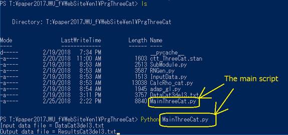
Figure 9
Listing 2. Stan script for items of three categories
// Yasuharu
Okamoto, 2017.07
data {
int <lower = 3, upper =
3> K;
//
Number of categories = 3
int Npsn;
//
Number of persons
int Nitm;
//
Number of items
int Ntot;
//
Number of data, Ntot <=
Nprn * Nitm
int<lower = 1, upper =
Npsn> IDpsn[Ntot]; // Person ID
int<lower = 1, upper =
Nitm> IDitm[Ntot]; // Item ID
int<lower = 1, upper =
K> Res[Ntot];
//
Response-> An integer value between 1 and K
}
parameters {
real<lower = 0.0> Lambda[Nitm];
real
mu[Nitm];
real<lower = 0.0> psi[Nitm];
real
F[Npsn];
}
transformed parameters
{
vector[K] p[Ntot];
real C[K - 1];
C[1] = -1.0;
C[2] = 1.0;
for (i in 1:Ntot){
p[i][K] = Phi(((mu[IDitm[i]] + (Lambda[IDitm[i]] * F[IDpsn[i]])) - C[K -
1]) /
psi[IDitm[i]]);
p[i][1] =1.0 - Phi(((mu[IDitm[i]] + (Lambda[IDitm[i]] * F[IDpsn[i]])) -
C[1]) /
psi[IDitm[i]]);
for (k
in 2:(K - 1)){
p[i][k] = Phi(((mu[IDitm[i]] + (Lambda[IDitm[i]] * F[IDpsn[i]])) - C[k -
1]) /
psi[IDitm[i]])
- Phi(((mu[IDitm[i]] + (Lambda[IDitm[i]] * F[IDpsn[i]])) - C[k]) /
psi[IDitm[i]]);
}
}
}
model {
for (i in 1:Npsn)
F[i]
~ normal(0.0, 1.0);
for (i in 1:Ntot)
Res[i] ~ categorical(p[i]);
}
(C)
Items
with two categories (Binary items)
For binary items, there is only one category boundary. So, restriction (13) cannot be used. In this case, the origin is set by the following condition
![]()
Under this condition (14), we have
![]()
![]()
![]()
![]()
where
![]()
Equation (15) shows that for binary items, parameters can be estimated under condition (14) and
![]()
Condition (16) sets the units of the items (Okamoto, 2017).
The Stan script for binary items is shown in Listing 3. The Stan script file and the Python script files are archived in a zip file with a sample data file. Hot to use the script is explained by a document (a pdf file).
The Python scripts can be run in the same way as in the case of items of more than three categories (see Figure 10).
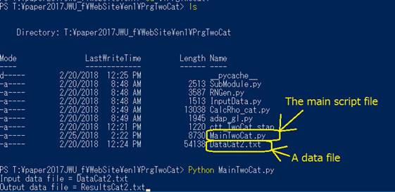
Figure 10
Listing 3. Stan script for binary items
// Yasuharu
Okamoto, 2017.07
data {
int <lower = 2, upper =
2> K;
//
Number of categories = 2
int Npsn;
//
Number of persons
int Nitm;
//
Number of items
int Ntot;
//
Number of data, Ntot <=
Nprn * Nitm
int<lower = 1, upper =
Npsn> IDpsn[Ntot]; // Person ID
int<lower = 1, upper =
Nitm> IDitm[Ntot]; // Item ID
int<lower = 1, upper =
K> Res[Ntot];
//
Response-> An integer value between 1 and K
}
parameters {
real<lower
= 0.0> Lambda[Nitm];
real
mu[Nitm];
real
F[Npsn];
}
transformed parameters
{
vector[K] p[Ntot];
real C[K - 1];
real psi[Nitm];
C[1] = 0.0;
for (j in 1:Nitm){
psi[j] = 1.0;
}
for (i in 1:Ntot){
p[i][K] = Phi(((mu[IDitm[i]] + (Lambda[IDitm[i]] * F[IDpsn[i]])) - C[K -
1]) /
psi[IDitm[i]]);
p[i][1] =1.0 - p[i][K];
}
}
model {
for (i in 1:Npsn)
F[i]
~ normal(0.0, 1.0);
for (i in 1:Ntot)
Res[i] ~ categorical(p[i]);
}
Godfrey-Smith, P. (2021). Theory and reality: An introduction to the philosophy of science, second edition. The University of Chicago Press.