Preprocessing of Categorical Variables by Common
Quantification
2023.11: Revised
Machine learning uses One-Hot-encoding to preprocess categorical variables. One-Hot-encoding constructs dummy variables for each value of categorical variables. On the other hand, common quantification assigns values to categorical values so that variance of the categorical variable with respect to the assigned values becomes (locally) maximum and (locally) maximum information in the categorical variable is obtained (Okamoto, 2015: body of the text is written in English).
Consider the following example of categorical variables (Table 1).
=================================================
Table 1. Data with a categorical variable CatV.
ID CatV
A1 alpha
A2 alpha
A3 gamma
A4 alpha
A5 alpha
B1 alpha
B2 alpha
B3 alpha
B4 gamma
C1 beta
C2 beta
C3 gamma
C4 beta
D1 beta
D2 beta
D3 beta
D4 gamma
=================================================
Categorical variables can be given numerical values by the
proposed quantification. For example, in Table 1, quantification, by which
categories alpha, beta, and gamma are given numerical values![]() ,
, ![]() , and
, and ![]() ,
respectively, is represented by the following equation.
,
respectively, is represented by the following equation.

Quantification values ![]() s can be
given by the following way:
s can be
given by the following way:
Set

then we have

![]() is called an
indicator matrix.
is called an
indicator matrix.
Set
![]()
then we have
![]()
Under the condition
![]()
we seek the ![]() , which
maximizes variance
, which
maximizes variance
![]()
This ![]() can be given
as an eigen vector
can be given
as an eigen vector ![]() in the following spectral decomposition
equation
in the following spectral decomposition
equation
![]()
where matrix ![]() is the
centered matrix of
is the
centered matrix of ![]()
![]()
When ![]() and
and ![]() are solution for eq. (1), then
are solution for eq. (1), then ![]() and
and ![]() are also solution for eq. (1). Hence, when
we calculate quantification, we may get weights, which are sign inverted. Both
weights are correct ones.
are also solution for eq. (1). Hence, when
we calculate quantification, we may get weights, which are sign inverted. Both
weights are correct ones.
For detailes about the quantification, see Okamoto (2015), the body of
which is written in English.
Programs and sample data files are archived into commonqfiles.zip.
The programs and data files in the archived file commonqfiles.zip
can be freely used by the reader.
In the following, How to use the program,
Example1 (PCA and regression analysis) and Example 2 (PCA and
cross tabulation) of the application are presented.
The main script, which is shown in Listing
1, calls the function common_q of mymodule.py, which is shown in Listing 2. Listings 1 and 2 are shown at the end of the
website.
To run the program, execute the command
PS D:\******\commonqfiles> python MainCommonQ.py
When the program starts, the input data file name is asked
PS
D:\******\commonqfiles> python MainCommonQ.py
Data
File Name (*.xlsx) =
The input data file is an Excel file, as shown in Figure
1.1.

Figure 1.1 File name: Data.xlsx
In the first row, variable names are set. The second row
indicates how to process the values of each variable. 0 indicates no
transformation, 1 means that standardization of the variable will be done, and
integer K larger than 1 means that the number of categories of that variable is
K and quantification of the variable is required. Data values are set from the
third row.
Set an input Excel data file name. If you use the file shown
in Figure 1.1, set as follows:
Data File Name (*.xlsx) = Data.xlsx
After the input data file name is set, the program processes
the data. When the program ends, the terminal shows messages like the
following:
PS
D:******\commonqfiles> python .\MainCommonQ.py
Data
File Name (*.xlsx) = Data.xlsx
ndata
= 17
nvar
= 6
indx
=
['GrpID' 'ID' 'Score' 'Attr.' 'CA' 'CB']
cndtn
=
[0 0 0 1 3 3]
Quantified
Data was saved in cq_Data.xlsx
Log
file = q_Data.txt
PS
D:******\commonqfiles>
The quantified data was saved as an Excel file of the file
name with prefix “cq_” to the input data file name.
Open this file, you can see the one shown in Figure 1.2 in
the case of the input data file shown in Figure 1.1.

Figure 1.2 Processed file: cq_Data.xlsx
Compare Figure 1.2 with Figure 1.1. Standardized variable
Attr is given the name Attr_z with suffix to the variable name. Quantified
variables CA and CB have prefix “q_”, each of which
has suffix like “_i”. The
suffix “_i” is added to the
i-th quantification variable with i starting from 0.
Open the log file, q_Data.txt, the name of which is shown in
the terminal after the program ended. The name of the log file is one with the
prefix “q_” to the input data file name, and the
file extension is replaced by “.txt”.
In the log file, you can see the values of weights for
quantification as follows:
Data
file = Data.xlsx
Quantification
of CA
eigen
values = [6.49239444 4.56642909]
Created...q_CA_0 for lambda = 6.4924
with omega = 0.74653
-0.65965 -0.08688
Created...q_CA_1 for lambda = 4.5664
with omega = -0.33069
-0.48117 0.81186
Quantification
of CB
eigen
values = [6.49239444 4.56642909]
Created...q_CB_0 for lambda = 6.4924
with omega = 0.74653
-0.65965 -0.08688
Created...q_CB_1 for lambda = 4.5664
with omega = -0.33069
-0.48117 0.81186
Output
file = cq_Data.xlsx
Example
1. Categorical variable and continuous variable
Data in Figure 2.1 is hypothetical data, with variables
DataID, species, and p_length.
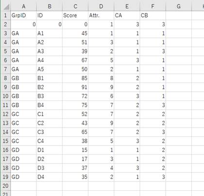
Figure 2.1 Hypothetical data.
To prepare for quantification of the categorical variable
species, categories Virginia, versicolor, and setosa are replaced by integers
1, 2, and 3. The quantification program assumes that categorical variable takes
an integer value from 1 to K when the number of categories is K. Correspondence
between the category and an integer is arbitrary, that is, categories are
considered in the nominal scale.
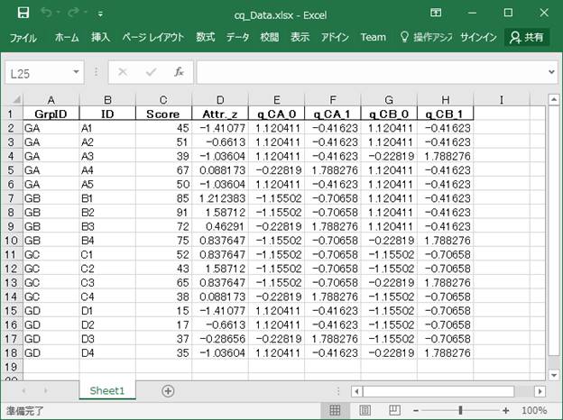
Figure 2.2 Data file for
quantification
Quantification of the data in Figure 2.2 gives the results
shown in Figure 2.3.
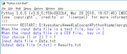
Figure 2.3 Quantification of the
data in Figure 2.2
Content of the log file is as follows:
Data
file = Data_irisK_1.xlsx
Quantification
of species
eigen
values = [3.6 3. ]
Created...q_species_0 for lambda = 3.6
with omega = 0.8165
-0.40825 -0.40825
Created...q_species_1 for lambda = 3.0
with omega = -4.1869e-16
-0.70711 0.70711
Output
file = cq_Data_irisK_1.xlsx
Analyze the three variables, q_species_0, q_species_1, and
p_length_z, by principal component analysis (PCA), then we get the results
shown in Figure 2.4. PCA may produce a sign inverted solution. Both solutions
are correct
Figure 2.4 Result of PCA
We see that q_species_0 and p_length_z have some relationship.
Analyze relation of variables q_species_0 and p_length_z by simple regression
model, then we get the result shown in Figure 2.5.
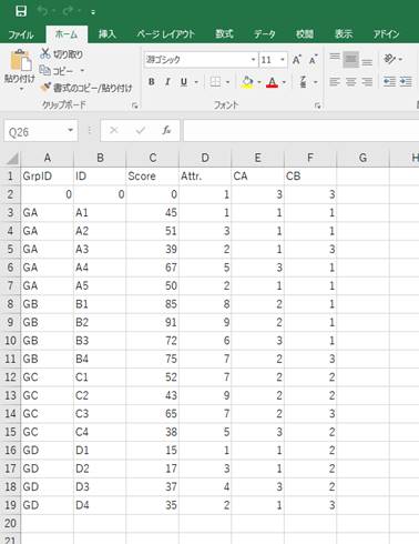
Figure 2.5 Regression analysis
In Figure 2.5, small random fluctuations are added to the
horizontal coordinates to avoid overlapping of points.
Quantification q_species_0 represents
Virginia, versicolor and setosa by weights 0.8165, -0.40824 and -0.40824 (See
the log file shown above). Figure 2.5 shows that p_length_z has larger values
for Virginia than for versicolor and setosa.
Exa,ple
2. Two categorical variables
Hypothetical data of eye color and hair color is shown in
Figure 3.1.
Figure 3.1 Hypothetical data
To quantify categorical data, categories Blue, Brown and
Hazel of eye colors are replaced by integers 1, 2, and 3, and Black, Bluenette,
and Red are replaced by integers 1, 2, and 3 (Figure 3.2). Quantification
program assumes that categorical variable takes an integer value from 1 to K
when the number of categories is K. Correspondence between the category and an
integer is arbitrary.

Figure 3.2 Data file for quantification
The results of quantification of the data in Figure 3.2 is
shown in Figure 3.3.

Figure 3.3 Quantification of the data in Figure 3.2
Content of the log file is as follows:
Data
file = Data_ColorK.xlsx
Quantification
of Eye
eigen
values = [3.88102497 2.31897503]
Created...q_Eye_0 for lambda = 3.881
with
omega = 0.59554 -0.7815 0.18596
Created...q_Eye_1 for lambda = 2.319
with omega = -0.55856
-0.23647 0.79504
Quantification
of Hair
eigen
values = [3.88102497 2.31897503]
Created...q_Hair_0 for lambda = 3.881
with omega = -0.18596
-0.59554 0.7815
Created...q_Hair_1 for lambda = 2.319
with omega = -0.79504
0.55856 0.23647
Output
file = cq_Data_ColorK.xlsx
PCA of the quantified data in Figure 3.3 gives the results
in Figure 3.4. PCA may produce a sign inverted solution. Both solutions are
correct.

Figure 3.4 PCA
Quantifications q_Eye_1 and q_Hair_0 look to be closely
related, and q_Eye_0 and q_Hair_1 also look to be closely related.
As an example, consider relation between q_Eye_1 and
q_Hair_0.
Construct a cross table of q_Eye_1 and q_Hair_0 by the
following script:
import
pandas as pd
import
numpy as np
with
pd.ExcelFile('Data_Color.xlsx') as xlsx:
data = pd.read_excel(xlsx)
xt
= pd.crosstab(np.array(data['Eye']), np.array(data['Hair']),
rownames = ['Eye'], colnames = ['Hair'])
print('\nCross
Table(DataFrame) =\n', xt)
xt
= np.array(xt)
print('\nCross
Table(nparray) =\n', xt)
w_eye_1
= [-0.55856, -0.23647, 0.79504]
w_hair_0
= [-0.18596, -0.59554, 0.7815]
idx_eye_1
= np.argsort(w_eye_1)
idx_hair_0
= np.argsort(w_hair_0)
print('\nw_eye_1
=\n', w_eye_1)
print('\nidx_eye_1
=\n', idx_eye_1)
print('w_hair_0
|n', w_hair_0)
print('idx_hair_0
=\n', idx_hair_0)
s_xt
= xt[idx_eye_1][:,idx_hair_0]
print('\nRearranged
Cross Table =\n', s_xt)
Run the script, then the following output is displayed on
the terminal
Cross
Table(DataFrame) =
Hair Black Bluenette Red
Eye
Blue 0
3 0
Brown 2
0 3
Hazel 0
0 2
Cross
Table(nparray) =
[[0 3 0]
[2 0 3]
[0 0 2]]
w_eye_1
=
[-0.55856, -0.23647, 0.79504]
idx_eye_1
=
[0 1 2]
w_hair_0
|n [-0.18596, -0.59554, 0.7815]
idx_hair_0
=
[1 0 2]
Rearranged
Cross Table =
[[3 0 0]
[0 2 3]
[0 0 2]]
Rows and Columns of the cross table created by pandas are
ordered alphabetically. After rearranging rows and columns according to weights
for the variables, the relation between the variables becomes to be seen more
clearly.
Reference
Okamoto,
Y. (2015). A Two-Step Analysis with Common Quantification of Categorical Data. Japan Women’s University Journal: Faculty of
Integrated Arts and Social Sciences, 26, 99-112 (Body of
the text is written in English).
Listing 1 Main script MainCommonQ.py
import
pandas as pd
import
scipy.stats as ss
import
numpy as np
import
mymodule as mm
flnm
= input('Data File Name (*.xlsx) = ')
fout_nm
= 'q_' + flnm[:-4] + 'txt'
fout
= open(fout_nm, 'w')
fout.write('Data
file = ' + flnm)
xlsx
= pd.ExcelFile(flnm)
data
= pd.read_excel(xlsx)
X
= data.values[1:]
ndata
= len(X)
print('ndata
= ', ndata)
indx
= data.columns.values
cndtn
= data.values[0]
nvar
= len(indx)
print('nvar
= ', nvar)
print('indx
=\n', indx)
print('cndtn
=\n', cndtn)
temp_df
= pd.DataFrame()
for
i in range(nvar):
if (cndtn[i] < 0):
print('condition for var-{} < 0'.format(i))
raise 'var_cond error.'
else:
if
(cndtn[i] == 0):
temp_df[indx[i]] = X[:, i]
elif
(cndtn[i] == 1):
temp_df[indx[i] + '_z'] = ss.zscore([x for x in X[:, i]])
else:
nq, varnames, qvars = mm.common_q(cndtn[i], indx[i], X[:, i], fout)
for j in range(nq):
temp_df[varnames[j]] = qvars[j]
with pd.ExcelWriter('cq_' + flnm) as
xl_writer:
temp_df.to_excel(xl_writer,
index = False)
print('\nQuantified
Data was saved in ' + 'cq_' + flnm)
fout.write('\n\nOutput
file = ' + 'cq_' + flnm)
fout.close()
print('\nLog
file = ' + fout_nm + '\n')
import
numpy as np
import
scipy as sc
def
common_q(K, vname, X, fout):
fout.write('\n\nQuantification
of {}'.format(vname))
nq = K - 1
n = len(X)
G = np.zeros((n, K))
for i in range(n):
G[i,
X[i] - 1] = 1.0
f = G.sum(axis = 0)
for k in range(K):
if
f[k] == 0:
print('Category-{0} of variable {1} is not used.'.format(k+1, vname))
fout.write('\n\nCategory-{0} of variable {1} is not used.'.format(k+1,
vname))
fout.close()
raise Exception('Category Error !')
One_n = np.ones((n, 1))
f = np.reshape(f, (1, K))
H = G - One_n @ f / n
HpH = H.T @ H
wt, vctr =
np.linalg.eig(HpH)
ck_idx = np.abs(wt) >
1.0e-7
wt = wt[ck_idx]
vctr = vctr[:, ck_idx]
idx = np.argsort(-wt)
wt = wt[idx]
vctr = vctr.T[idx].T
fout.write('\neigen values =
{}'.format(wt))
nq = len(wt)
qnames = []
qvars = []
for h in range(nq): #K - 1):
qnames.append('q_' + vname + '_{}'.format(h))
z =
H @ np.reshape(vctr[:,h], (K, 1)) / ((wt[h]/n) ** 0.5)
qvars.append(z)
fout.write('\nCreated...{0:s}
for lambda = {1:.5}\n'.format(qnames[-1], wt[h]))
fout.write('
with omega = ')
for
j in range(K):
fout.write('{0:.5}
'.format(vctr[j][h]))
return nq, qnames, qvars