Bayesian Analysis for Psychometric Functions
Two-, three-, and four-alternative procedures
The programs in this website can be used freely on user’s responsibility, although all rights are reserved.
Yasuharu Okamoto
Models are described first, and then programs are explained.
Models
Two-alternative
procedure
A comparison stimulus ![]() is compared with the
standard stimulus
is compared with the
standard stimulus ![]() , and judgment “Which is stronger?” is required. The probability that
, and judgment “Which is stronger?” is required. The probability that ![]() is judged to be stronger
than
is judged to be stronger
than ![]() is denoted by
is denoted by ![]() . In a two-alternative procedure, an observer chooses one of two
judgments,
. In a two-alternative procedure, an observer chooses one of two
judgments, ![]() (
(![]() is stronger than
is stronger than ![]() ) and
) and ![]() (
(![]() is weaker than
is weaker than ![]() ), so the probability
), so the probability ![]() is given by
is given by
![]()
![]() can be considered to be
a function of
can be considered to be
a function of ![]() and is called a
psychometric function (PF). A psychometric function is usually well
approximated by a cumulative normal distribution (phi-gamma hypothesis; see
Luce and Galanter, 1963). Hence, set
and is called a
psychometric function (PF). A psychometric function is usually well
approximated by a cumulative normal distribution (phi-gamma hypothesis; see
Luce and Galanter, 1963). Hence, set
![]()
where ![]() is the cumulative
standard normal distribution.
is the cumulative
standard normal distribution.
The point of subjective equality PSE is given by
![]()
Just noticeable difference JND is given by
![]()
where discrimination probability 0.75 is
chosen for JND. ![]() satisfies the equation
satisfies the equation
![]()
Denote the comparison stimulus and its judgment
in trial ![]() by
by ![]() and
and ![]() , where
, where
![]()
Then the probability of the data is given by
![]()
where
![]()
Based on probability (2), the posterior distributions are given. To estimate the posterior distribution, the programs in this website uses MCMC algorithms.
Three-alternative
procedure
Three alternative procedure allows “don’t know” or “indifferent” judgment as an additional judgment to the two-alternative procedure (Böckenholt, 2001; Kaernbach, 2001). Hence, the three categories of judgments are as follows
![]() : which means that
: which means that ![]() is judged to be weaker
than
is judged to be weaker
than ![]()
![]() : which means that
: which means that ![]() is judged to equal
is judged to equal ![]()
![]() : which means that
: which means that ![]() is judged to be stronger
than
is judged to be stronger
than ![]()
Combine the two categories ![]() and
and ![]() into one category, which
is denoted by
into one category, which
is denoted by ![]() .
.
Set the following two PFs
![]()
![]()
Then we have
![]()
and
![]()
JND is given by
![]()
Assuming that C1 and C2 are at an equal distance from PSE, we have
![]()
Okamoto (2012) reported an experimental result, which showed assumption (3) does not always hold. In his experiment, four-alternative procedure was used to test assumption (3).
Denote the comparison stimulus and its
judgment in trial ![]() by
by ![]() and
and ![]() , where
, where

Then the probability of the data is given by
![]()
where

Based on probability (4), the posterior distributions are given. To estimate the posterior distribution, the programs in this website uses MCMC algorithms.
Four-alternative
procedure
A four-alternative procedure allows four response categories:
![]() : which means that
: which means that ![]() is judged to be weaker
than
is judged to be weaker
than ![]()
![]() : which means that
: which means that ![]() is probably weaker than
is probably weaker than ![]()
![]() : which means that
: which means that ![]() is probably stronger
than
is probably stronger
than ![]()
![]() : which means that
: which means that ![]() is judged to be stronger
than
is judged to be stronger
than ![]()
Combine the three response categories ![]() ,
, ![]() , and
, and ![]() into one category, which
is denoted by
into one category, which
is denoted by ![]() .
.
Combine the two categories ![]() and
and ![]() into one category, which
is denoted by
into one category, which
is denoted by ![]() , and the two categories
, and the two categories ![]() and
and ![]() into one category, which
is denoted by
into one category, which
is denoted by ![]() .
.
Combine the three categories ![]() ,
, ![]() , and
, and ![]() into one category, which
is denoted by
into one category, which
is denoted by ![]() .
.
Then, set the following three PFs
![]()
![]()
![]()
We have the following probabilities
![]()
![]()
![]()
PSE is given by
![]()
and JND is given by
![]()
Denote the comparison stimulus and its
judgment in trial ![]() by
by ![]() and
and ![]() , where
, where

Then the probability of the data is given by
![]()
where

Based on probability (5), the posterior distributions are given. To estimate the posterior distribution, the programs in this website uses MCMC algorithms.
Experimental
Design
For the method of constant stimuli, width
of intervals between comparison stimuli may be as wide as three times of JND.
Range of the comparison stimuli should be wide enough so that all response categories
are used by the observer. However, the set of the comparison stimuli is not
required to include stimuli, for which the probabilities of judgments ![]() and
and ![]() are 1 or 0, because the
analysis is based on Bayesian methods.
are 1 or 0, because the
analysis is based on Bayesian methods.
For an adapting method, width of intervals between comparison stimuli need not be very small, because the analysis is based on Bayesian methods. About twice of JND would work. Okamoto (2012) used an adapting method for a four-alternative procedure, which is an extension of the psi method.
On Fechner’s Problem
Relation between thresholds and scales of sensation is discussed as Fechner’s problem. Models related to this are discussed in Okamoto (2001, 2005).
References
Böckenholt,U. (2001). Threshold and intransitivities in pairwise judgments: A multilevel analysis. Journal of Educational and Behavioral Sciences, 26, 269-282.
Kaernbach, C. (2001). Adaptive threshold estimation with unforced-choice tasks. Perception & Psychophysics, 63, 1377-1388.
Luce, R. D. & Galanter, E. (1963). Discrimination. In P. Suppes, J. L. Zinnes, R. R. Bush, E. Galanter, R.D. Luce, W. J. McGill, A. Newell, and H. A. Simon (Eds.), Handbook of Mathematical Psychology: Vol. I (pp. 191-243). New York: John Wiley and Sons, Inc.
Programs
Two-alternative
procedure
The program files and a sample data file for two-alternative procedure are archived into the file PM2Cat.zip. Run the program mainprg.py, then the name of the input data file is asked (Figure 1).

Figure 1
The format of the data file is shown in Figure 2.

![]()
![]()
![]()

Figure 2
The data are written after the line with
slash / at the head. Each line of the data includes a set of dataID, ![]() , and
, and ![]() in each trial. DataID is
simply any string and used to identify the set, but is not used in analysis.
After the last data, a line with slash / at the head is put to indicate the end
of the data.
in each trial. DataID is
simply any string and used to identify the set, but is not used in analysis.
After the last data, a line with slash / at the head is put to indicate the end
of the data.
After the input data file name is set and the Enter key is pressed down, then an output text file name is asked. Set a text file name, then calculation starts.

Figure 3
When calculation ends (Figure 3), a window, in which the PF is drawn, is displayed (Figure 4).

Figure 4
Small green circles represent data points ![]() . To avoid overlapping of circles, small random fluctuations are
added to get the drawn points
. To avoid overlapping of circles, small random fluctuations are
added to get the drawn points ![]() , where
, where
![]()
![]() is a small random
fluctuation.
is a small random
fluctuation.
After closing the window in Figure 4, the
next window, in which a histogram of samples for PSE (![]() ) is drawn, will be displayed (Figure 5).
) is drawn, will be displayed (Figure 5).
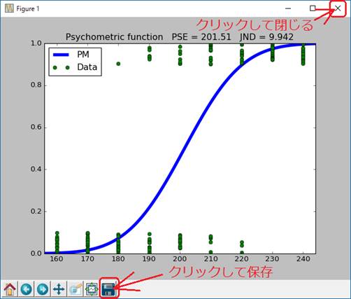
Figure 5
After the window in Figure 5 is closed, the window, in which a histogram for JND is drawn, is displayed (Figure 6).

Figure 6
Closing the window in Figure 6, the program ends (Figure 7).

Figure 7
After the program ends, the output file can be opened by an editor. Figure 8 shows the contents of the output file.

・
・
・

Figure 8
At the end of the file, medians, quartile points, and 95% CIs are written.
The main source code file mainprg.py, which is included in the archived file PM2Cat.zip, is shown below.
=============== mainprg.py ===================
from
multiprocessing.pool import Pool
import math
from mcmcFunc import *
from RNGen import *
from subprg import *
#
# Yasuharu
Okamoto, 2016.11
#
if __name__ ==
'__main__':
X, n, meanSt, sgmSt, fout,
nm_fout = InputData()
NSimu = 1000
params = {'jump' : 0,
'n' : n,
'X' : X,
'NSimu' : NSimu,
'initMu' : meanSt,
'initSgm' : sgmSt,
'genSgmMu' : sgmSt/10.0,
'genSgmSgm' :
sgmSt/10.0}
#
# Adjust the
parameters in MCMC
#
istep = 0
while True:
print("\nStep-{} started.".format(istep))
Mu,
Sgm, cnt_mu, cnt_sgm = mcmcFunc( params )
sum_mu = 0.0
sum_sgm
= 0.0
for
t in range(1, NSimu + 1):
sum_mu += Mu[t]
sum_sgm += Sgm[t]
params['initMu'] = sum_mu / NSimu
params['initSgm'] = sum_sgm / NSimu
print("meanMu = {}".format(params['initMu']))
print("meanSgm =
{}".format(params['initSgm']))
ck_cnt = 0
r_mu
= cnt_mu / NSimu
print("r_mu = {}".format(r_mu))
v,
ck_cnt = scale_sgm( r_mu, ck_cnt )
params['genSgmMu'] = params['genSgmMu'] * v
print("genSgmMu
= {}".format(params['genSgmMu']))
r_sgm = cnt_sgm / NSimu;
print("r_sgm = {}".format(r_sgm))
v,
ck_cnt = scale_sgm( r_sgm, ck_cnt )
params['genSgmSgm'] = params['genSgmSgm'] * v
print("genSgmSgm = {}".format(params['genSgmSgm']))
print("ck_cnt = {}".format(ck_cnt))
if
ck_cnt == 0:
break
istep += 1
#
#
The main MCMCs
#
NSimu = 3000
params['NSimu'] = NSimu
n_mcmc = 4
ary_params = []
for i in range(0, n_mcmc):
temp
= params.copy()
temp['jump'] = i + 1
ary_params.append(temp)
print("\nThe main MCMCs
started.")
pool = Pool()
results = pool.map(mcmcFunc,
ary_params) # Multiprocessing
print("\nThe main MCMCs
ended.\n")
mrg_mu = []
mrg_sgm = []
for temp_Mu, temp_Sgm,
cnt_mu, cnt_sgm in results:
mrg_mu += temp_Mu[1:NSimu + 1]
mrg_sgm += temp_Sgm[1:NSimu + 1]
print("Length(mrg_mu) =
{}".format(len(mrg_mu)))
print("Length(mrg_sgm)
= {}".format(len(mrg_sgm)))
mrg_mu.sort()
mrg_sgm.sort()
DispResults( NSimu, n_mcmc,
X, n, mrg_mu, mrg_sgm, fout)
fout.close()
print("\nOutput file {}
was saved.".format(nm_fout))
==================================
The program uses multiprocessing for MCMC. Output by the print function of child processes can be seen when the program is run in a console window (Figure 9).

Figure 9
Three-alternative
procedure
The program files and a sample data file for three-alternative procedure are archived into the file PM3Cat.zip. Run the program mainprg3Cat.py, then the name of the input data file is asked (Figure 10).

Figure 10
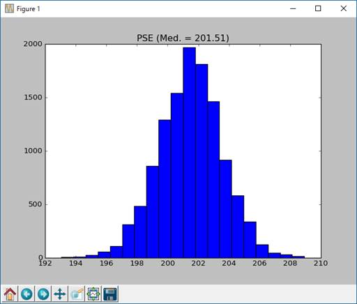
The format of the data file is shown in Figure 11.
・
・
・
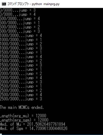
Figure 11
The data are written after the line with slash / at the head. Each line of the data includes a set of dataID, S_comp, and Res in each trial. DataID is simply any string and used to identify the set, but is not used in analysis. After the last data, a line with slash / at the head is put to indicate the end of the data.
After the input data file name is set and the Enter key is pressed down, then an output text file name is asked. Set a text file name, then calculation starts.
When calculation ends, a window, in which the two PFs are drawn, is displayed (Figure 12).
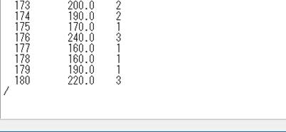
Figure 12
Small green circles represent data points ![]() . To avoid overlapping of circles, small random fluctuations are
added to get the drawn points
. To avoid overlapping of circles, small random fluctuations are
added to get the drawn points ![]() , where
, where

![]() is a small random
fluctuation.
is a small random
fluctuation.
After closing the window in Figure 12, the next window, in which frequency polygons of samples for C1 and C2 are drawn, will be displayed (Figure 13).
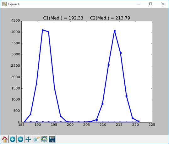
Figure 13
After the window in Figure 13 is closed, the window, in which a histogram for JND is drawn, is displayed (Figure 14).
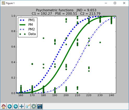
Figure 14
Closing the window in Figure 14, the program ends.
After the program ends, the output file can be opened by an editor. Figure 15 shows the contents of the output file.

・
・
・
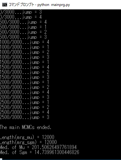
Figure 15
At the end of the file, medians, quartile points, and 95% CIs for C1, C2 and JND are written.
The main source code file mainprg3Cat.py, which is included in the archived file PM3Cat.zip, is shown below.
============== mainprg3Cat.py ===================
from
multiprocessing.pool import Pool
import
matplotlib.pyplot as plt
import numpy as np
import math
from mcmcFunc3Cat
import *
from RNGen import *
from subprg import *
#
# Yasuharu
Okamoto, 2016.11
#
if __name__ ==
'__main__':
X, n, meanSt, sgmSt, fout,
nm_fout = InputData()
NSimu = 1000
params = {'jump' : 0,
'n' : n,
'X' : X,
'NSimu' : NSimu,
'initC1' : meanSt - sgmSt,
'initC2' : meanSt + sgmSt,
'initSgm' : sgmSt,
'genSgmC1' : sgmSt/10.0,
'genSgmC2'
: sgmSt/10.0,
'genSgmSgm' : sgmSt/10.0}
#
#
Adjust the parameters in MCMC
#
istep = 0
while True:
print("Step-{} started.".format(istep))
C1,
C2, Sgm, cnt_C1, cnt_C2, cnt_sgm = mcmcFunc( params )
sum_C1 = 0.0
sum_C2 = 0.0
sum_sgm = 0.0
for
t in range(1, NSimu + 1):
sum_C1 += C1[t]
sum_C2 += C2[t]
sum_sgm += Sgm[t]
params['initC1'] = sum_C1 / NSimu
params['initC2'] = sum_C2 / NSimu
params['initSgm'] = sum_sgm / NSimu
print("meanC1 = {}".format(params['initC1']))
print('meanC2 = {}'.format(params['initC2']))
print("meanSgm = {}".format(params['initSgm']))
ck_cnt = 0
r_C1
= cnt_C1 / NSimu
print("r_C1 = {}".format(r_C1))
v,
ck_cnt = scale_sgm( r_C1, ck_cnt )
params['genSgmC1'] = params['genSgmC1'] * v
print("genSgmC1 = {}".format(params['genSgmC1']))
r_C2
= cnt_C2 / NSimu
print("r_C2 = {}".format(r_C2))
v,
ck_cnt = scale_sgm( r_C2, ck_cnt )
params['genSgmC2'] = params['genSgmC2'] * v
print("genSgmC2 = {}".format(params['genSgmC2']))
r_sgm = cnt_sgm / NSimu;
print("r_sgm = {}".format(r_sgm))
v,
ck_cnt = scale_sgm( r_sgm, ck_cnt )
params['genSgmSgm'] = params['genSgmSgm'] * v
print("genSgmSgm = {}".format(params['genSgmSgm']))
print("ck_cnt = {}".format(ck_cnt))
if
ck_cnt == 0:
break
istep += 1
#
#
The main MCMCs
#
NSimu = 3000
params['NSimu'] = NSimu
n_mcmc = 4
ary_params = []
for i in range(0, n_mcmc):
temp
= params.copy()
temp['jump'] = i + 1
ary_params.append(temp)
print("\nThe main MCMCs
started.")
pool = Pool()
results = pool.map(mcmcFunc,
ary_params)
print("\nThe main MCMCs
ended.")
mrg_C1 = []
mrg_C2 = []
mrg_sgm = []
for temp_C1, temp_C2,
temp_Sgm, cnt_C1, cnt_C2, cnt_sgm in results:
mrg_C1 += temp_C1[1:NSimu + 1]
mrg_C2 += temp_C2[1:NSimu + 1]
mrg_sgm += temp_Sgm[1:NSimu + 1]
print("Length(mrg_C1) =
{}".format(len(mrg_C1)))
print('Length(mrg_C2) =
{}'.format(len(mrg_C2)))
print("Length(mrg_sgm)
= {}".format(len(mrg_sgm)))
mrg_C1.sort()
mrg_C2.sort()
mrg_sgm.sort()
DispResults( NSimu, n_mcmc,
X, n, mrg_C1, mrg_C2, mrg_sgm, fout )
fout.close()
print("\nOutput file {}
was saved.".format(nm_fout))
====================================
Four-alternative
procedure
The program files and a sample data file for four-alternative procedure are archived into the file PM4Cat.zip. Run the program mainprg4Cat.py, then the name of the input data file is asked (Figure 16).

Figure 16
The format of the data file is shown in Figure 17.
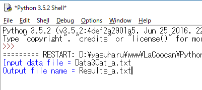
・
・
・

Figure 17
The data are written after the line with slash / at the head. Each line of the data includes a set of dataID, S_comp, and Res in each trial. DataID is simply any string and used to identify the set, but is not used in analysis. After the last data, a line with slash / at the head is put to indicate the end of the data.
After the input data file name is set and the Enter key is pressed down, then an output text file name is asked. Set a text file name, then calculation starts.
When calculation ends, a window, in which the three PFs are drawn, is displayed (Figure 18).

Figure 18
Small green circles represent data points ![]() . To avoid overlapping of circles, small random fluctuations are
added to get the drawn points
. To avoid overlapping of circles, small random fluctuations are
added to get the drawn points ![]() , where
, where
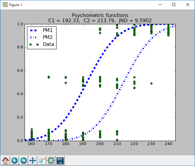
![]() is a small random
fluctuation.
is a small random
fluctuation.
After closing the window in Figure 18, the next window, in which frequency polygons of samples for C1, PSE, and C2 are drawn, will be displayed (Figure 19).
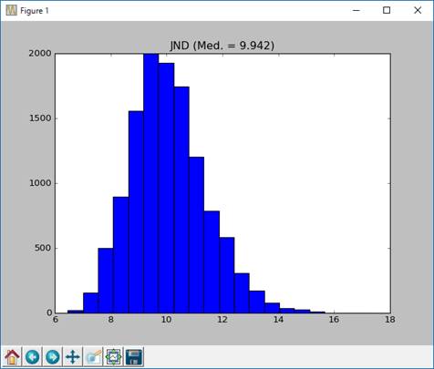
Figure 19
After the window in Figure 19 is closed, the window, in which a histogram for JND is drawn, is displayed (Figure 20).
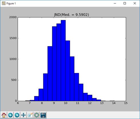
Figure 20
Closing the window in Figure 20, the program ends.
After the program ends, the output file can be opened by an editor. Figure 21 shows the contents of the output file.

Figure 21
At the end of the file, medians, quartile points, and 95% CIs for C1, PSE, C2 and JND are written.
The main source code file mainprg4Cat.py, which is included in the archived file PM4Cat.zip , is shown below.
============== mainprg4Cat.py ===================
from
multiprocessing.pool import Pool
from mcmcFunc4Cat
import *
from subprgs4Cat import
*
#
# Yasuharu
Okamoto, 2016.11
#
if __name__ ==
'__main__':
X, n, meanSt, sgmSt, fout,
nm_fout = InputData()
NSimu = 1000
params = {'jump' : 0,
'n' : n,
'X' : X,
'NSimu' : NSimu,
'initC1' : meanSt - sgmSt,
'initMu' : meanSt,
'initC2' : meanSt + sgmSt,
'initSgm' : sgmSt,
'genSgmC1' : sgmSt/10.0,
'genSgmMu' : sgmSt / 10.0,
'genSgmC2' : sgmSt/10.0,
'genSgmSgm' : sgmSt/10.0}
istep = 0
while True:
print("Step-{} started.".format(istep))
C1,
Mu, C2, Sgm, cnt_C1, cnt_Mu, cnt_C2, cnt_sgm = mcmcFunc( params )
sum_C1 = 0.0
sum_Mu
= 0.0
sum_C2 = 0.0
sum_sgm = 0.0
for
t in range(1, NSimu + 1):
sum_C1 += C1[t]
sum_Mu += Mu[t]
sum_C2 += C2[t]
sum_sgm += Sgm[t]
params['initC1'] = sum_C1 / NSimu
params['initMu'] = sum_Mu / NSimu
params['initC2'] = sum_C2 / NSimu
params['initSgm'] = sum_sgm / NSimu
print("meanC1 = {}".format(params['initC1']))
print("meanMu = {}".format(params['initMu']))
print('meanC2 = {}'.format(params['initC2']))
print("meanSgm = {}".format(params['initSgm']))
ck_cnt = 0
r_C1
= cnt_C1 / NSimu
print("r_C1 = {}".format(r_C1))
v,
ck_cnt = scale_sgm( r_C1, ck_cnt )
params['genSgmC1'] = params['genSgmC1'] * v
print("genSgmC1 = {}".format(params['genSgmC1']))
r_Mu
= cnt_Mu / NSimu
print('r_Mu = {}'.format(r_Mu))
v,
ck_cnt = scale_sgm( r_Mu, ck_cnt )
params['genSgmMu'] = params['genSgmMu'] * v
print("genSgmMu = {}".format(params['genSgmMu']))
r_C2
= cnt_C2 / NSimu
print("r_C2 = {}".format(r_C2))
v,
ck_cnt = scale_sgm( r_C2, ck_cnt )
params['genSgmC2'] = params['genSgmC2'] * v
print("genSgmC2 = {}".format(params['genSgmC2']))
r_sgm = cnt_sgm / NSimu;
print("r_sgm = {}".format(r_sgm))
v,
ck_cnt = scale_sgm( r_sgm, ck_cnt )
params['genSgmSgm'] = params['genSgmSgm'] * v
print("genSgmSgm = {}".format(params['genSgmSgm']))
print("ck_cnt = {}".format(ck_cnt))
if
ck_cnt == 0:
break
istep += 1
NSimu = 3000
params['NSimu'] = NSimu
n_mcmc = 4
ary_params = []
for i in range(0, n_mcmc):
temp
= params.copy()
temp['jump'] = i + 1
ary_params.append(temp)
print("\nThe main MCMCs
started.")
pool = Pool()
results = pool.map(mcmcFunc,
ary_params)
print("\nThe main MCMCs
ended.")
mrg_C1 = []
mrg_Mu = []
mrg_C2 = []
mrg_sgm = []
for temp_C1, temp_Mu,
temp_C2, temp_Sgm, cnt_C1, cnt_Mu, cnt_C2, cnt_sgm in results:
mrg_C1 += temp_C1[1:NSimu + 1]
mrg_Mu += temp_Mu[1:NSimu + 1]
mrg_C2 += temp_C2[1:NSimu + 1]
mrg_sgm += temp_Sgm[1:NSimu + 1]
print("Length(mrg_C1) =
{}".format(len(mrg_C1)))
print("Length(mrg_Mu) =
{}".format(len(mrg_Mu)))
print('Length(mrg_C2) =
{}'.format(len(mrg_C2)))
print("Length(mrg_sgm)
= {}".format(len(mrg_sgm)))
mrg_C1.sort()
mrg_Mu.sort()
mrg_C2.sort()
mrg_sgm.sort()
DispResults( NSimu, n_mcmc,
X, n, mrg_C1, mrg_Mu, mrg_C2, mrg_sgm, fout )
fout.close()
print("\nOutput file {}
was saved.".format(nm_fout))
======================================