カテゴリ評定尺度法
2026.06改訂
刺激の感覚の強さを順序カテゴリで答え、それに基づいて尺度を構成する方法は、カテゴリ尺度法(Gescheider, 1997, p. 214)、評定尺度法(難波・桑野、1998, pp. 72-86)、あるいは継次カテゴリ法/系列カテゴリ法(method of successive categories)(岡本、2006、pp. 27-36)、継次間隔法(method of successive intervals)(中谷、1969, p. 162)などと呼ばれている。カテゴリ尺度法では、評定を順序尺度のレベルの日常語で行うことができる。評定カテゴリが主観的に等間隔でなければならないという制約はない。順序尺度であればよい。このとき、数理モデルを設定すれば量的分析が可能である(岡本、2025)。例えば、刺激の感覚量とカテゴリ境界の関係にThurstone(1927)の判断の基本モデルを適用したカテゴリ判断の法則(The law of categorical judgment; Torgerson, 1958p. 205)を用いて分析することができる。なお、刺激値は区別されておればよい、すなわち、名義尺度のレベルであればよい。刺激の感覚量は、数理モデルによる分析により与えられる。
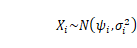
提示された刺激 の感覚の強さをK個の順序付けられたカテゴリから選んで答えるものとする。刺激の引き起こす感覚量を確率変数
 で表し、平均
 、標準偏差
、標準偏差 の正規分布に従うものとする。すなわち、
である。
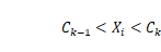
感覚の連続体上におけるK個のカテゴリの境界を で、評価カテゴリを
 で表すとき、
 のとき
のとき 
とする。
このとき、刺激の感覚がカテゴリ であると判断される確率は、

である。ここで、 は累積標準正規分布関数である。
感覚連続体の原点と単位を決めるために、カテゴリ境界の両端を0と1に設定する。
 、
、 
感覚の強さの範囲(ダイナミックレンジ)が刺激の種類に依らずほぼ同じであるという仮定(Teghtsoonian, 1971)に従えば、この制約条件は自然なものである。
感覚の標準偏差については、以下の3つの場合を想定した。
F条件: 標準偏差に特に制約条件を設定しない。
L条件: 標準偏差に制約条件

を設定する。これはStevens(1975, p. 235)がEkmanの法則と呼んでいるものを踏まえたものである。
C条件: 標準偏差は全て等しく

とする場合。これは、Fechnerの考え方に対応するものである。
上記3条件に対応してPythonプログラムを3通り作成した。これらのプログラムとデータ例のファイルは圧縮ファイルcatscalfiles.zipにまとめた。
3つのプログラムの入力データの形式はすべて同じである。例を図1に示す。
第1行目は、変数名である。2行目からデータを、1列目に提示刺激、2列目から各評価カテゴリの頻度を入力する。

図1
カテゴリは、左から順番に強さに対応するように並べる。例えば、音の強さであれば、「ほとんど聞こえない」、・・・、「非常に強い」などである。
刺激は、上の行から順番に並べる。強さの小さいものから順番に並べておくとグラフは見やすくなる。社会的・文化的刺激のように強さの順序が明確でない場合は刺激の値の強さの順に並べる必要はない。刺激の感覚量の強さは、本ウェブサイトのプログラムによる分析で得られる。大きさの順に並べておく方が、分析結果は見やすいので、分析後、あらためて並べなおせばよい。分析の結果やには影響しない。刺激値を横軸に取ったときのグラフは、第1列に設定された数値が横軸の値になるので、刺激値と感覚量が単調関係にあると、見やすいグラフになる。刺激値に対する感覚量は、スクリプトの出力ファイルを見れば分かる。
1列目は、数値を入力する。文字列を設定すると、読み込み時にエラーになる。
分析は、個々の刺激とカテゴリの関係がデータ全体の文脈において分析される。刺激間の感覚量の関係が不明なときは、とりあえず適当に数値を与えておいて、分析後、グラフが見易くなるように数値を入れ替えればよい。このとき、入れ替えた数値が昇順になるように行の入れ替えも行うと、データファイルが見易くなる。。
図1のように作成したデータを、CSV形式で保存する。CSV形式のファイルは、Excelの場合、保存ファイル名のファイル拡張子として.csv選ぶとCSV形式で保存される。
以下に、F条件、L条件、C条件のプログラムについて順番に説明する。感覚強度が強くなると感覚の変動が大きくなると考えられるときはL条件、感覚の強度にかかわらず感覚の強さの変動は一定であると考えられるときはC条件、感覚の強さと変動の大きさが不明のときはF条件のプログラムを試してみればよい。F条件での分析結果の結果、感覚が強くなると変動が大きくなる傾向が見られれば、L条件での分析を試みればよい。感覚の強さにかかわらず変動が同じであればC条件での分析を試みればよい。
標準偏差に制約条件を置かないときのベイズ分析のStanスクリプトをリストF1に示すように用意した。
リストF1のStanスクリプトを利用するPythonスクリプトはリストF2のように用意した。
ファイルは、catscalfiles.zipにまとめた。
リストF1のファイル(RatingFree.stan)、リストF2のファイル(cscalefree.py)、および入力データファイルを同じフォルダに置く。そのフォルダにカレントディレクトリ(フォルダ)を移して、CmdStanPyがインストールされた環境において、次のコマンドを実行する。CmdStanPyの簡単な解説を、このウェブサイトにおいて行った。
(stan) *****/SigmaFree$ python cscalefree.py
上のコマンドを実行すると、入力データファイル名を聞いてくる。
(stan) *****/SigmaFree$
python cscalefree.py
Input file (*.csv) = DataC.csv
上の例では、入力データファイル名としてDataC.csvを設定している。これは、図F1に示すものである。データの設定形式については、図1の説明を参照されたい。

図F1
入力データファイル名を設定すると、ファイルが読み込まれ、Stanスクリプトのコンパイルが始まる。コンパイルには多少時間が掛かる。コンパイル後、MCMCサンプリングが始まり、サンプリングが終了すると、図F2のグラフが表示される。

図F2
感覚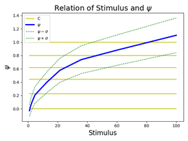 の事後分布のグラフである。
図F2のWindowを閉じると、図F3のグラフが表示される。

図F3
感覚の標準偏差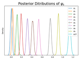 の事後分布のグラフである。事後分布が重なっているので、標準偏差が等しい、すなわち等分散であることが示唆されていると思われる。
図F3のWindowを閉じると、図F4のグラフが表示される。

図F4
横軸に感覚の事後分布の中央値を取り、縦軸に対応する感覚の標準偏差の事後分布の中央値と第1四分位数および第3四分位数を表示したものである。
感覚と標準偏差の間に明瞭な関係は認められない。
図F4のWindowを閉じると、図F5のグラフが表示される。

図F5
カテゴリ境界 の事後分布のグラフである。両端の分布が棒になっているのは、
 、
、 の仮定が置かれているからである。
図F5のWindowを閉じると、図F6のグラフが表示される。

図F6
刺激値と感覚の関係が描かれている。グラフが単調増加関数でないときは、データ(図F1)の刺激値の値を感覚と単調関係にあるように設定しなおせばよい。刺激値と感覚の値は、出力ファイルに出力される。刺激値の再設定を行ったときは、行を入れ替えて、データの配列(図F1)において刺激値が昇順に並ぶようにする。
図F6のWindowを閉じると、図F7のグラフが表示される。

図F7
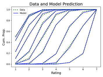
各刺激値における評定カテゴリのデータおよびモデルの累積曲線である。モデルの累積曲線は、パラメータの事後分布の中央値をパラメータの点推定値(Gelmanら、2021)として描かれている。
図F7のWindowを閉じると、実行終了である。
実行終了後、出力ファイルResults.txtを開くと以下のようになっている。
Input Data File = DataC.csv
Data:
1 51 36 13 0 0 0 0
1.668 43 46 10 1 0 0 0
2.783 23 48 27 2 0 0 0
4.642 10 44 36 10 0 0 0
7.743 1 21 54 22 2 0 0
12.915 0 11 37 42 9 1 0
21.544 0 0 23 49 25 3 0
35.938 0 0 0 19 49 28 4
59.948 0 0 0 1 32 37 30
100 0 0 0 0 3 16 81
Stimulus Med.
Psi Med. Sigma
1.00
-0.00
0.20
1.67
0.03
0.18
2.78
0.13
0.18
4.64
0.22
0.18
7.74
0.35
0.16
12.91
0.46
0.17
21.54
0.58
0.15
35.94
0.80
0.13
59.95
0.93
0.13
100.00
1.14
0.15
刺激(Stimulus)に対する感覚(Med. Psi)が記されている。
他の入力データファイルの分析
比較のために他の入力データファイルを分析してみる。
(stan) ****/SigmaFree$
python cscalefree.py
Input file (*.csv) = DataL.csv
上の例では、入力データファイルDataL.csvを指定している。
この入力データファイルのときは、図F4に対応するグラフが下図のようになる。

図F4a
明らかに感覚と標準偏差の間に強い関係が認められる。
リストF1 F条件の場合のStanスクリプト(RatingFree.stan)
functions {
real my_phi(real
x) {
if (x <= -37.5) {
return 0.0;
}
else
if (x >= 8.25) {
return 1.0;
}
else
{
return std_normal_cdf(x);
}
}
}
data {
int NSt;
int K;
array[NSt]
real Sts;
array[NSt,
K] int Rs;
}
transformed data {
vector[K-2] a_C;
for (i
in 1:(K-2)) {
a_C[i] = 1.0;
}
}
parameters {
array[NSt]
real<lower = 0.001, upper=10.0> sgms;
simplex[K-2] preC;
array[NSt]
real<lower=-10, upper=10> Psis;
}
transformed parameters {
array[K-1] real C;
array[NSt]
simplex[K] theta;
real v;
C[1] = 0.0;
C[K-1] = 1.0;
v = 0.0;
for (k in 2:(K-2)) {
v =
v + preC[k-1];
C[k]
= C[1] + v;
}
for (s in 1:NSt) {
theta[s][1] = my_phi((C[1] - Psis[s]) / sgms[s]);
theta[s][K] = 1.0 - my_phi((C[K-1] - Psis[s]) / sgms[s]);
for
(k in 2:(K-1)) {
theta[s][k] = my_phi((C[k] - Psis[s]) / sgms[s]) -
my_phi((C[k-1] - Psis[s])
/ sgms[s]);
}
for
(k in 1:K) {
theta[s][k] = (1.0e-9)/K + (theta[s][k] * (1 - 1.0e-9));
}
}
}
model {
for (s in 1:NSt) {
sgms[s] ~ uniform(0.001, 10.0);
}
for (s in 1:NSt) {
Psis[s] ~ uniform(-10, 10);
}
preC
~ dirichlet(a_C);
for (s in 1:NSt) {
Rs[s] ~ multinomial(theta[s]);
}
}
リストF2 F条件のベイズ分析Pythonスクリプト(cscalefree.py)
import csv
import numpy
as np
from cmdstanpy
import CmdStanModel
import matplotlib.pyplot
as plt
import seaborn as sb
import scipy.stats
as ss
fout = open('Results.txt', 'w')
fin_nm = input('Input file (*.csv) = ')
with open(fin_nm,
'r') as f:
Data_in
= [v for v in csv.reader(f)]
fout.write('Input Data File = {}\n'.format(fin_nm))
NSt = len(Data_in) - 1
K = len(Data_in[0]) - 1
Sts = np.empty(NSt)
Rs = np.empty((NSt, K), dtype = 'int')
for j in range(NSt):
Sts[j]
= float(Data_in[j+1][0])
for k
in range(K):
Rs[j][k] = int(Data_in[j+1][k+1])
fout.write('\nData:\n')
for j in range(NSt):
print(f'{Sts[j]:>10g}',
end = '')
fout.write(f'{Sts[j]:>10g}')
for k
in range(K):
print(f'{Rs[j][k]:>5d}', end = '')
fout.write(f'{Rs[j][k]:>5d}')
print()
fout.write('\n')
Data = {'NSt':NSt, 'K':K, 'Sts':Sts, 'Rs':Rs}
model = CmdStanModel(stan_file='RatingFree.stan')
fit = model.sample(data=Data,
adapt_delta=1.0-1.0e-12, max_treedepth=15,
iter_warmup=5000, iter_sampling=2000)
print(fit.summary())
df_fit = fit.draws_pd()
# PandasのDataFrame
Psis = []
for i in
range(NSt):
Psis.append(df_fit[f'Psis[{i+1}]'])
Psis = np.array(Psis).T
sgms = []
for i in
range(NSt):
sgms.append(df_fit[f'sgms[{i+1}]'])
sgms = np.array(sgms).T
Cs = []
for i in
range(K-1):
Cs.append(df_fit[f'C[{i+1}]'])
Cs = np.array(Cs).T
for i in
range(NSt):
sb.kdeplot(Psis.T[i], label =
r'$\psi_{}$'.format(i+1))
plt.title(r'Posterior
Ditributions of $\psi_s$', fontsize = 20)
plt.yticks([])
plt.legend()
plt.tight_layout()
plt.savefig('FigPsiPost.png')
plt.show()
for i in
range(NSt):
sb.kdeplot(sgms.T[i], label =
r'$\sigma_{}$'.format(i))
plt.title(r'Posterior
Distributions of $\sigma_s$', fontsize
= 20)
plt.legend()
plt.savefig('FigSgmPost.png')
plt.show()
Psis_med = np.median(Psis, axis=0)
sgms_q1q2q3 = np.percentile(sgms, [25,50,75], axis=0)
print(sgms_q1q2q3)
for i in
range(len(Psis_med)):
plt.plot([Psis_med[i], Psis_med[i]], [sgms_q1q2q3[0][i],
sgms_q1q2q3[2][i]],
'-', lw=2, color='g')
plt.plot(Psis_med,
sgms_q1q2q3[1], 'o', color='b', label='Median')
plt.xlabel('$\\psi$', fontsize=16)
plt.ylabel('$\\sigma$', fontsize=16)
plt.legend()
plt.show()
plt.plot([0, 0], [0, 5], label = r'$C_0$')
for i in
range(1, K-2):
sb.kdeplot(Cs.T[i], label = r'$C_{}$'.format(i+1))
plt.plot([1,1], [0, 5], label = r'$C_{}$'.format(K-1))
plt.title('Posterior Distributions of Cs', fontsize = 20)
plt.yticks([])
plt.legend()
plt.savefig('FigCsPost.png')
plt.show()
v_psis = np.empty(NSt)
v_sgms = np.empty(NSt)
for i in
range(NSt):
v_psis[i] = np.median(Psis.T[i])
v_sgms[i] = np.median(sgms.T[i])
fout.write('\n{0:>15s}{1:>15s}{2:>15s}\n'.format(
'Stimulus', 'Med. Psi', 'Med. Sigma'))
for vst, vpsi, vsgm in zip(Sts, v_psis, v_sgms):
fout.write('{0:>15.2f}{1:>15.2f}{2:>15.2f}\n'.format(vst, vpsi, vsgm))
v_Cs = np.empty(K-1)
v_Cs[0] = 0.0
v_Cs[K-2] = 1.0
for k in range(1, K-2):
v_Cs[k]
= np.median(Cs.T[k])
for k in range(K-1):
plt.plot([Sts[0], Sts[-1]], [v_Cs[k], v_Cs[k]], color = 'y')
plt.plot([], 'y-', label = 'C')
plt.plot(Sts, v_psis, color = 'b', lw = 3,
label = r'$\psi$')
plt.plot(Sts, v_psis - v_sgms, color = 'g',
linestyle = '--', lw
= 1,label = r'$\psi - \sigma$')
plt.plot(Sts, v_psis + v_sgms, color = 'g',
linestyle = '--', lw
= 1, label = r'$\psi+ \sigma$')
plt.xlabel('Stimulus', fontsize
= 16)
plt.ylabel(r'$\psi$', fontsize
= 16)
plt.legend(loc = 'upper left')
plt.title(r'Relation
of Stimulus and $\psi$', fontsize = 18)
plt.tight_layout()
plt.savefig('PsiSgmC.png')
plt.show()
Probs = np.empty((NSt, K))
for s in range(NSt):
Probs[s][0] = ss.norm(loc = v_psis[s], scale = v_sgms[s]).cdf(v_Cs[0])
Probs[s][K-1] = 1.0 - ss.norm(loc = v_psis[s], scale = v_sgms[s]).cdf(v_Cs[K-2])
for k
in range(1, K-1):
Probs[s][k] = ss.norm(loc = v_psis[s], scale = v_sgms[s]).cdf(v_Cs[k]) -\
ss.norm(loc = v_psis[s],
scale = v_sgms[s]).cdf(v_Cs[k-1])
print('Predicted Prob(Rating|Stimulus):')
for s in range(NSt):
for k
in range(K):
print(f'
{Probs[s][k]:7.3f}', end = '')
print()
Pred_Rs = np.empty((NSt, K))
N_Rs = np.sum(Rs,
axis = 1)
for i in
range(NSt):
Pred_Rs[i] = N_Rs[i] * Probs[i]
print('Predicted Frequencies of Rating
for Stimulus:')
for s in range(NSt):
for k
in range(K):
print(f' {Pred_Rs[s][k]:7.1f}', end = '')
print()
cum_data_Rs = np.cumsum(Rs,
axis = 1)
cum_pred_Rs = np.cumsum(Pred_Rs, axis = 1)
print(cum_data_Rs)
for s in range(NSt):
if s == 0:
plt.plot(range(K), cum_data_Rs[s]/cum_data_Rs[s][K-1], 'g:',
lw = 3, label = 'Data')
else:
plt.plot(range(K), cum_data_Rs[s]/cum_data_Rs[s][K-1], 'g:',
lw = 3 )
if s == 0:
plt.plot(range(K), cum_pred_Rs[s]/cum_pred_Rs[s][K-1], 'b-',
label = 'Model')
else:
plt.plot(range(K), cum_pred_Rs[s]/cum_pred_Rs[s][K-1], 'b-')
plt.xticks(range(K), range(1, K+1))
plt.xlabel('Rating', fontsize
= 14)
plt.ylabel('Cum. Prop.', fontsize
= 14)
plt.legend()
plt.title('Data and Model Prediction', fontsize = 18)
plt.tight_layout()
plt.savefig('FigDataModel.png')
plt.show()
fout.close()
感覚の標準偏差が感覚の1次関数として増加するというL条件のベイズ分析を行うStanスクリプトをリストL1のように作成した。
リストL1のStanスクリプトを用いてベイズ分析を行うPythonスクリプトをリストL2のように用意した。
リストL1のファイル(RatingEkman.stan)、リストL2のファイル(cscalelinear.py)、および入力データファイルを同じフォルダに置く。そのフォルダにカレントディレクトリ(フォルダ)を移して、CmdStanPyのインストールされた環境で次のコマンドを実行する。CmdStanPyについては、このウェブサイトに簡単な説明を用意した。
(stan) *****/SigmaLinear$ python cscalelinear.py
上のコマンドを実行すると、入力データファイル名の設定が求められる。
(stan) *****/SigmaLinear$
python cscalelinear.py
Input file (*.csv) = DataL.csv
入力データファイルは、図L1に示す形式のファイルを設定する。ファイルのデータの設定形式は、図1の説明を参照されたい。

図L1
上のコマンドの例では、入力データファイル名として図L1のものが設定されている。
入力データファイル名を設定すると、ファイルが読み込まれ、Stanスクリプトのコンパイルが始まる。コンパイル後、MCMCサンプリングが行われ、サンプリングが終了すると、図L2のグラフが表示される。

図L2
感覚の事後分布のグラフである。
図L2のWindowを閉じると、図L3のグラフが表示される。

図L3
感覚の標準偏差の事後分布のグラフである。L条件であるので、事後分布は刺激値に応じてシフトしているのが分かる。
図L3のWindowを閉じると、図L4のグラフが表示される。

図L4
カテゴリ境界の事後分布のグラフである。両端の分布が棒になっているのは、、の仮定が置かれているからである。
図L5のWindowを閉じると、図L6のグラフが表示される。

図L6
パラメータ と
と の事後分布のグラフである。
L条件の式
は、Stanスクリプト(リストL1)では、以下のようにコーディングされている。
min_psi
= min(Psis);
max_psi
= max(Psis);
for (s in 1:NSt) {
sgms[s] = sgm0 + a * (Psis[s] - min_psi) / (max_psi - min_psi);
}
これは、標準偏差が正の値であるという制限内で、感覚との線形性を保つためである。
図L6のWindowを閉じると、図L7のグラフが表示される。

図L7
刺激値と感覚の関係が描かれている。グラフが単調増加関数でないときは、データ(図L1)の刺激値の値を感覚と単調関係にあるように設定しなおせばよい。刺激値と感覚の値は、出力ファイルに出力される。刺激値の再設定を行ったときは、行を入れ替えて、データの配列(図L1)において刺激値が昇順に並ぶようにする。
図L7のWindowを閉じると、図L8のグラフが表示される。

図L8
各刺激値における評定カテゴリのデータおよびモデルの累積曲線である。モデルの累積曲線は、パラメータの事後分布の中央値をパラメータの点推定値(Gelmanら、2021)として描かれている。
図L8のWindowを閉じると、実行終了である。
実行終了後、出力ファイルResults.txtを開くと以下のようになっている。
Input Data File = DataL.csv
Data:
1 63 37 0 0 0 0 0
1.668 33 65 2 0 0 0 0
2.783 18 67 15 0 0 0 0
4.642 4 53 40 3 0 0 0
7.743 3 28 56 13 0 0 0
12.915 1 13 45 30 11 0 0
21.544 0 3 21 34 33 8 1
35.938 0 0 8 20 36 25 11
59.948 0 0 1 15 21 32 31
100 0 0 0 2 7 26 65
Stimulus Med.
Psi Med. Sigma
1.00
-0.02
0.08
1.67
0.04
0.09
2.78
0.10
0.12
4.64
0.21
0.12
7.74
0.29
0.14
12.91
0.41
0.17
21.54
0.58
0.19
35.94
0.75
0.21
59.95
0.89
0.23
100.00
1.09
0.21
刺激値(Stimulus)と感覚(Med Psi)が出力されている。感覚は事後分布の中央値である(Gelmanら、2021)。
リストL1 L条件のStanスクリプト(RatingEkman.stan)
functions {
real my_phi(real
x) {
if
(x <= -37.5) {
return 0.0;
}
else
if (x >= 8.25) {
return 1.0;
}
else
{
return std_normal_cdf(x);
}
}
}
data {
int NSt;
int K;
array[NSt]
real Sts;
array[NSt,
K] int Rs;
}
transformed data {
vector[K-2] a_C;
for (i
in 1:(K-2)) {
a_C[i] = 1.0;
}
}
parameters {
array[NSt]
real Psis;
simplex[K-2] preC;
real<lower=0.01,
upper=10.0> sgm0;
real<lower=0.01,
upper=10.0> a;
}
transformed parameters {
array[NSt]
real sgms;
array[K-1] real C;
array[NSt]
simplex[K] theta;
real min_psi;
real max_psi;
real v;
min_psi
= min(Psis);
max_psi
= max(Psis);
for (s in 1:NSt) {
sgms[s] = sgm0 + a * (Psis[s] - min_psi) / (max_psi - min_psi);
}
C[1] = 0.0;
C[K-1] = 1.0;
v = 0.0;
for (k in 2:(K-2)) {
v =
v + preC[k-1];
C[k]
= C[1] + v;
}
for (s in 1:NSt) {
theta[s][1] = my_phi((C[1] - Psis[s]) / sgms[s]);
theta[s][K] = 1.0 - my_phi((C[K-1] - Psis[s]) / sgms[s]);
for
(k in 2:(K-1)) {
theta[s][k] = my_phi((C[k] - Psis[s]) / sgms[s]) -
my_phi((C[k-1] - Psis[s])
/ sgms[s]);
}
for
(k in 1:K) {
theta[s][k] = (1.0e-9)/K + (theta[s][k] * (1 - 1.0e-9));
}
}
}
model {
preC
~ dirichlet(a_C);
sgm0 ~ uniform(0.01, 10.0);
a ~ uniform(0.01, 10.0);
for (s in 1:NSt) {
Psis[s] ~ uniform(-10.0, 10.0);
Rs[s] ~ multinomial(theta[s]);
}
}
リストL2 L条件でのベイズ分析Pythonスクリプト(cscalelinear.py)
from cmdstanpy
import CmdStanModel
import csv
import numpy
as np
import matplotlib.pyplot
as plt
import seaborn as sb
import scipy.stats
as ss
fout = open('Results.txt', 'w')
fin_nm = input('Input file (*.csv) = ')
with open(fin_nm,
'r') as f:
Data_in
= [v for v in csv.reader(f)]
fout.write('Input Data File = {}\n'.format(fin_nm))
NSt = len(Data_in) - 1
K = len(Data_in[0]) - 1
Sts = np.empty(NSt)
Rs = np.empty((NSt, K), dtype = 'int')
for j in range(NSt):
Sts[j]
= float(Data_in[j+1][0])
for k
in range(K):
Rs[j][k] = int(Data_in[j+1][k+1])
fout.write('\nData:\n')
for j in range(NSt):
print(f'{Sts[j]:>10g}',
end = '')
fout.write(f'{Sts[j]:>10g}')
for k
in range(K):
print(f'{Rs[j][k]:>5d}', end = '')
fout.write(f'{Rs[j][k]:>5d}')
print()
fout.write('\n')
Data = {'NSt':NSt, 'K':K, 'Sts':Sts, 'Rs':Rs}
model = CmdStanModel(stan_file='RatingEkman.stan')
fit = model.sample(data=Data,
adapt_delta=0.9999, max_treedepth=15,
iter_warmup=5000, iter_sampling=2000)
print(fit.summary())
df_fit = fit.draws_pd()
# PandasのDataFrame型に変換
Psis = []
for i in
range(NSt):
Psis.append(df_fit[f'Psis[{i+1}]'])
Psis = np.array(Psis).T
sgms = []
for i in
range(NSt):
sgms.append(df_fit[f'sgms[{i+1}]'])
sgms = np.array(sgms).T
Cs = []
for i in
range(K-1):
Cs.append(df_fit[f'C[{i+1}]'])
Cs = np.array(Cs).T
sgm0 = df_fit['sgm0']
a = df_fit['a']
for i in
range(NSt):
sb.kdeplot(Psis.T[i], label =
r'$\psi_{}$'.format(i+1))
plt.title(r'Posterior
Ditributions of $\psi_s$', fontsize = 20)
plt.yticks([])
plt.legend()
plt.tight_layout()
plt.savefig('FigPsiPost.png')
plt.show()
for i in
range(NSt):
sb.kdeplot(sgms.T[i], label = r'$\sigma_{}$'.format(i))
plt.title(r'Posterior
Distributions of $\sigma_s$', fontsize
= 20)
plt.legend()
plt.savefig('FigSgmPost.png')
plt.show()
plt.plot([0, 0], [0, 5], label = r'$C_0$')
for i in
range(1, K-2):
sb.kdeplot(Cs.T[i], label = r'$C_{}$'.format(i+1))
plt.plot([1,1], [0, 5], label = r'$C_{}$'.format(K-1))
plt.title('Posterior Distributions of Cs', fontsize = 20)
plt.yticks([])
plt.legend()
plt.savefig('FigCsPost.png')
plt.show()
med_sgm0 = np.median(sgm0)
med_a = np.median(a)
plt.figure(figsize =
(8,4))
plt.subplot(1,2,1)
sb.kdeplot(sgm0)
plt.yticks([])
plt.xlabel('sgm0', fontsize
= 14)
plt.title('Posterior Distribution of sgm0' +
'\nmed = {0:.2f}'.format(med_sgm0),
fontsize = 14)
plt.subplot(1,2,2)
sb.kdeplot(a)
plt.title('Posterior Distribtuion
of a' +
'\nmed = {0:.2f}'.format(med_a),
fontsize = 14)
plt.yticks([])
plt.xlabel('a', fontsize
= 14)
plt.tight_layout()
plt.savefig('Fig_a_b_Post.png')
plt.show()
v_psis = np.empty(NSt)
v_sgms = np.empty(NSt)
for i in
range(NSt):
v_psis[i] = np.median(Psis.T[i])
v_sgms[i] = np.median(sgms.T[i])
fout.write('\n{0:>15s}{1:>15s}{2:>15s}\n'.format(
'Stimulus', 'Med Psi', 'Med Sigma'))
for vst, vpsi, vsgm in zip(Sts, v_psis, v_sgms):
fout.write('{0:>15.2f}{1:>15.2f}{2:>15.2f}\n'.format(vst, vpsi, vsgm))
v_Cs = np.empty(K-1)
v_Cs[0] = 0.0
v_Cs[K-2] = 1.0
for k in range(1, K-2):
v_Cs[k]
= np.median(Cs.T[k])
for k in range(K-1):
plt.plot([Sts[0], Sts[-1]], [v_Cs[k], v_Cs[k]], color = 'y')
plt.plot([], 'y-', label = 'C')
plt.plot(Sts, v_psis, color = 'b', lw = 3,
label = r'$\psi$')
plt.plot(Sts, v_psis - v_sgms, color = 'g', linestyle = '--', lw = 1,
label = r'$\psi - \sigma$')
plt.plot(Sts, v_psis + v_sgms, color = 'g', linestyle = '--', lw = 1,
label = r'$\psi+ \sigma$')
plt.xlabel('Stimulus', fontsize
= 16)
plt.ylabel(r'$\psi$', fontsize
= 16)
plt.legend(loc = 'upper left')
plt.title(r'Relation
of Stimulus and $\psi$', fontsize = 18)
plt.tight_layout()
plt.savefig('PsiSgmC.png')
plt.show()
Probs = np.empty((NSt, K))
for s in range(NSt):
Probs[s][0] = ss.norm(loc = v_psis[s], scale = v_sgms[s]).cdf(v_Cs[0])
Probs[s][K-1] = 1.0 - ss.norm(loc = v_psis[s], scale = v_sgms[s]).cdf(v_Cs[K-2])
for k
in range(1, K-1):
Probs[s][k] = ss.norm(loc = v_psis[s], scale = v_sgms[s]).cdf(v_Cs[k]) -\
ss.norm(loc = v_psis[s],
scale = v_sgms[s]).cdf(v_Cs[k-1])
print('Predicted Prob(Rating|Stimulus):')
for s in range(NSt):
for k
in range(K):
print(f'
{Probs[s][k]:7.3f}', end = '')
print()
Pred_Rs = np.empty((NSt, K))
N_Rs = np.sum(Rs,
axis = 1)
for i in
range(NSt):
Pred_Rs[i] = N_Rs[i] * Probs[i]
print('Predicted Frequencies of Rating
for Stimulus:')
for s in range(NSt):
for k
in range(K):
print(f' {Pred_Rs[s][k]:7.1f}', end = '')
print()
cum_data_Rs = np.cumsum(Rs,
axis = 1)
cum_pred_Rs = np.cumsum(Pred_Rs, axis = 1)
print(cum_data_Rs)
for s in range(NSt):
if s == 0:
plt.plot(range(K), cum_data_Rs[s]/cum_data_Rs[s][K-1], 'g:', lw =
3, label = 'Data')
else:
plt.plot(range(K), cum_data_Rs[s]/cum_data_Rs[s][K-1], 'g:', lw = 3
)
if s == 0:
plt.plot(range(K), cum_pred_Rs[s]/cum_pred_Rs[s][K-1], 'b-', label = 'Model')
else:
plt.plot(range(K), cum_pred_Rs[s]/cum_pred_Rs[s][K-1], 'b-')
plt.xticks(range(K), range(1, K+1))
plt.xlabel('Rating', fontsize
= 14)
plt.ylabel('Cum. Prop.', fontsize
= 14)
plt.legend()
plt.title('Data and Model Prediction', fontsize = 18)
plt.tight_layout()
plt.savefig('FigDataModel.png')
plt.show()
fout.close()
print('\nResults.txt was saved.\n')
感覚の標準偏差が感覚の強さによらず一定であるC条件のStanスクリプトを、リストC1のように用意した。
リストC1のStanスクリプトを用いてベイズ分析を行うPythonスクリプトをリストC2のように用意した。
リストC1のファイル(RatingFechner.stan)、リストC2のファイル(cscaleconst.py)、および入力データファイルを同じフォルダに置く。そのフォルダにカレントディレクトリ(フォルダ)を移して、CmdStanPyのインストールされた環境において、次のコマンドを実行する。CmdStanPyについては、簡単な解説をこのウェブサイトに用意した。
(stan) *****/SigmaConst$ python cscaleconst.py
上のコマンドを実行すると、入力データファイル名の設定が求められる。
(stan) *****/SigmaConst$
python cscaleconst.py
Input file (*.csv) = DataC.csv
入力データファイルは、図C1に示す形式で用意する。図1の解説を参照されたい。

図C1
上のコマンドの例では、図C1のファイル名DataC.csvが設定されている。
入力データファイル名を設定すると、ファイルが読み込まれ、Stanスクリプトがコンパイルされる。このコンパイルには、多少時間が掛かる。コンパイルが終了すると、MCMCサンプリングが行われ、終了すると図C2のグラフが表示される。

図C2
感覚の事後分布のグラフである。
図C2のWindowを閉じると、図C3のグラフが表示される。

図C3
感覚の標準偏差の事後分布のグラフである。
図C3のWindowを閉じると、図C4のグラフが表示される。

図C4
カテゴリ境界の事後分布のグラフである。両端の分布が棒になっているのは、、の仮定が置かれているからである。
図C4のWindowを閉じると、図C5のグラフが表示される。

図C5
刺激値と感覚の関係が描かれている。グラフが単調増加関数でないときは、データ(図C1)の刺激値の値を感覚と単調関係にあるように設定し直せばよい。刺激値と感覚の値は、出力ファイルに出力される。刺激値の再設定を行ったときは、行を入れ替えて、データの配列(図C1)において刺激値が昇順に並ぶようにする。
図C5のWindowを閉じると、図C6のグラフが表示される。

図C6
各刺激値における評定カテゴリのデータおよびモデルの累積曲線である。モデルの累積曲線は、パラメータの事後分布の中央値をパラメータの点推定値(Gelmanら、2021)として算出されている。
図C6のWindowを閉じると、スクリプトの実行終了である。
実行終了後、出力ファイルResults.txtを開くと、以下のような内容である。
Input Data File = DataC.csv
Data:
1 51 36 13 0 0 0 0
1.668 43 46 10 1 0 0 0
2.783 23 48 27 2 0 0 0
4.642 10 44 36 10 0 0 0
7.743 1 21 54 22 2 0 0
12.915 0 11 37 42 9 1 0
21.544 0 0 23 49 25 3 0
35.938 0 0 0 19 49 28 4
59.948 0 0 0 1 32 37 30
100 0 0 0 0 3 16 81
Stimulus Med
Psi
1.00
0.01
1.67
0.03
2.78
0.11
4.64
0.20
7.74
0.31
12.91
0.42
21.54
0.54
35.94
0.76
59.95
0.92
100.00
1.13
Sigma: med =
0.15
刺激値(Stimulus)と感覚(Med Psi)が出力されている。
リストC1 C条件のStanスクリプト(RatingFechner.stan)
functions {
real my_phi(real
x) {
if
(x <= -37.5) {
return 0.0;
}
else
if (x >= 8.25) {
return 1.0;
}
else
{
return std_normal_cdf(x);
}
}
}
data {
int NSt;
int K;
array[NSt]
real Sts;
array[NSt,
K] int Rs;
}
transformed data {
vector[K-2] a_C;
for (i
in 1:(K-2)) {
a_C[i] = 1.0;
}
}
parameters {
array[NSt]
real<lower=0.0001, upper=10.0> Psis;
simplex[K-2] preC;
real<lower = 0.001,
upper=10.0> sgm;
}
transformed parameters {
array[K-1] real C;
array[NSt]
simplex[K] theta;
real v;
C[1] = 0.0;
C[K-1] = 1.0;
v = 0.0;
for (k in 2:(K-2)) {
v =
v + preC[k-1];
C[k]
= C[1] + v;
}
for (s in 1:NSt) {
theta[s][1] = my_phi((C[1] - Psis[s]) / sgm);
theta[s][K] = 1.0 - my_phi((C[K-1] - Psis[s]) / sgm);
for (k
in 2:(K-1)) {
theta[s][k] = my_phi((C[k] - Psis[s]) / sgm) -
my_phi((C[k-1] - Psis[s])
/ sgm);
}
for
(k in 1:K) {
theta[s][k] = (1.0e-9)/K + (theta[s][k] * (1 - 1.0e-9));
}
}
}
model {
preC
~ dirichlet(a_C);
sgm
~ uniform(0.001, 10.0);
for (s in 1:NSt) {
Psis[s] ~ uniform(0.0001, 10.0);
Rs[s] ~ multinomial(theta[s]);
}
}
リストC2 リストC1のStanスクリプトを用いるPythonスクリプト(cscaleconst.py)
from cmdstanpy
import CmdStanModel
import csv
import pandas as pd
import numpy
as np
import matplotlib.pyplot
as plt
import seaborn as sb
import scipy.stats
as ss
fout = open('Results.txt', 'w')
fin_nm = input('Input file (*.csv) = ')
with open(fin_nm,
'r') as f:
Data_in
= [v for v in csv.reader(f)]
fout.write('Input Data File = {}\n'.format(fin_nm))
NSt = len(Data_in) - 1
K = len(Data_in[0]) - 1
Sts = np.empty(NSt)
Rs = np.empty((NSt, K), dtype = 'int')
for j in range(NSt):
Sts[j]
= float(Data_in[j+1][0])
for k
in range(K):
Rs[j][k] = int(Data_in[j+1][k+1])
fout.write('\nData:\n')
for j in range(NSt):
print(f'{Sts[j]:>10g}',
end = '')
fout.write(f'{Sts[j]:>10g}')
for k
in range(K):
print(f'{Rs[j][k]:>5d}', end = '')
fout.write(f'{Rs[j][k]:>5d}')
print()
fout.write('\n')
Data = {'NSt':NSt, 'K':K, 'Sts':Sts, 'Rs':Rs}
model = CmdStanModel(stan_file='RatingFechner.stan')
fit = model.sample(data=Data)
print(fit.summary())
df_fit = fit.draws_pd()
# PandasのDataFrame型に変換
Psis = []
for i in
range(NSt):
Psis.append(df_fit[f'Psis[{i+1}]'])
Psis = np.array(Psis).T
sgm = np.array(df_fit['sgm'])
Cs = []
for i in
range(K-1):
Cs.append(df_fit[f'C[{i+1}]'])
Cs = np.array(Cs).T
for i in
range(NSt):
sb.kdeplot(Psis.T[i], label =
r'$\psi_{}$'.format(i+1))
plt.title(r'Posterior
Ditributions of $\psi_s$', fontsize = 20)
plt.yticks([])
plt.legend()
plt.tight_layout()
plt.savefig('FigPsiPost.png')
plt.show()
sb.kdeplot(sgm, label
= r'$\sigma$')
plt.title(r'Posterior
Distribution of $\sigma$', fontsize = 20)
plt.legend()
plt.savefig('FigSgmPost.png')
plt.show()
plt.plot([0, 0], [0, 5], label = r'$C_0$')
for i in
range(1, K-2):
sb.kdeplot(Cs.T[i], label = r'$C_{}$'.format(i+1))
plt.plot([1,1], [0, 5], label = r'$C_{}$'.format(K-1))
plt.title('Posterior Distributions of Cs', fontsize = 20)
plt.yticks([])
plt.legend()
plt.savefig('FigCsPost.png')
plt.show()
v_psis = np.empty(NSt)
for i in
range(NSt):
v_psis[i] = np.median(Psis.T[i])
v_sgm = np.median(sgm)
fout.write('\n{0:>15s}{1:>15s}\n'.format('Stimulus', 'Med Psi'))
for vst, vpsi in zip(Sts, v_psis):
fout.write('{0:>15.2f}{1:>15.2f}\n'.format(vst, vpsi))
fout.write('\nSigma:
med = {0:>15.2f}\n'.format(v_sgm))
v_Cs = np.empty(K-1)
v_Cs[0] = 0.0
v_Cs[K-2] = 1.0
for k in range(1, K-2):
v_Cs[k]
= np.median(Cs.T[k])
for k in range(K-1):
plt.plot([Sts[0], Sts[-1]], [v_Cs[k], v_Cs[k]], color = 'y')
plt.plot([], 'y-', label = 'C')
plt.plot(Sts, v_psis, color = 'b', lw = 3,
label = r'$\psi$')
plt.plot(Sts, v_psis - v_sgm, color = 'g', linestyle = '--', lw = 1,
label = r'$\psi - \sigma$')
plt.plot(Sts, v_psis + v_sgm, color = 'g', linestyle = '--', lw = 1,
label = r'$\psi+ \sigma$')
plt.xlabel('Stimulus', fontsize
= 16)
plt.ylabel(r'$\psi$', fontsize
= 16)
plt.legend(loc = 'upper left')
plt.title(r'Relation
of Stimulus and $\psi$', fontsize = 18)
plt.tight_layout()
plt.savefig('PsiSgmC.png')
plt.show()
Probs = np.empty((NSt, K))
for s in range(NSt):
Probs[s][0] = ss.norm(loc = v_psis[s], scale = v_sgm).cdf(v_Cs[0])
Probs[s][K-1] = 1.0 - ss.norm(loc = v_psis[s], scale = v_sgm).cdf(v_Cs[K-2])
for k
in range(1, K-1):
Probs[s][k] = ss.norm(loc = v_psis[s], scale = v_sgm).cdf(v_Cs[k]) -\
ss.norm(loc = v_psis[s],
scale = v_sgm).cdf(v_Cs[k-1])
print('Predicted Prob(Rating|Stimulus):')
for s in range(NSt):
for k
in range(K):
print(f'
{Probs[s][k]:7.3f}', end = '')
print()
Pred_Rs = np.empty((NSt, K))
N_Rs = np.sum(Rs,
axis = 1)
for i in
range(NSt):
Pred_Rs[i] = N_Rs[i] * Probs[i]
print('Predicted Frequencies of Rating
for Stimulus:')
for s in range(NSt):
for k
in range(K):
print(f' {Pred_Rs[s][k]:7.1f}', end = '')
print()
cum_data_Rs = np.cumsum(Rs,
axis = 1)
cum_pred_Rs = np.cumsum(Pred_Rs, axis = 1)
print(cum_data_Rs)
for s in range(NSt):
if s == 0:
plt.plot(range(K), cum_data_Rs[s]/cum_data_Rs[s][K-1], 'g:', lw =
3, label = 'Data')
else:
plt.plot(range(K), cum_data_Rs[s]/cum_data_Rs[s][K-1], 'g:', lw = 3
)
if s == 0:
plt.plot(range(K), cum_pred_Rs[s]/cum_pred_Rs[s][K-1], 'b-', label = 'Model')
else:
plt.plot(range(K), cum_pred_Rs[s]/cum_pred_Rs[s][K-1], 'b-')
plt.xticks(range(K), range(1, K+1))
plt.xlabel('Rating', fontsize
= 14)
plt.ylabel('Cum. Prop.', fontsize
= 14)
plt.legend()
plt.title('Data and Model Prediction', fontsize = 18)
plt.tight_layout()
plt.savefig('FigDataModel.png')
plt.show()
fout.close()
Gelman, A., Carlin, J. B., Stern, H. S., Dunson, D. B., Vehtari, A., & Rubin, D. B. (2014). Bayesian data analysis, 3rd. Ed. CRC Press.
Gelman, A., Hill, J., & Vehtari, A. (2021). Regression and other stories. Cambridge University
Gescheider, G. A. (1997). Psychophysics: The fundamentals, Third edition. Mahwah: Lawrence Erlbaum Associations, Publishers.
中谷和夫(1969).第5章 尺度構成法. 八木冕(監修)/田中良久(編)講座心理学2 計量心理学.東京大学出版会.
難波精一郎・桑野園子(1998).音の評価のための心理学的測定法.コロナ社.
岡本安晴(2006).計量心理学.培風館.
岡本安晴(2025).感覚・知覚測定法.和氣典二・重野純・村上郁也(編)感覚・知覚心理学ハンドブック 第三版(第2章)、誠信書房
Stevens, S. S. (1975). Psychophysics: Introduction to its perceptual, neural, and social prospects. New York: Wiley.
Tesghtsoonian, R. (1971). On the exponents in Stevens’ law and the constant in Ekman’s law. Psychological Review, 78, 71-80.
Thurstone, L. L. (1927). A law of comparative judgment. Psychological Review, 34, 273-286.
Torgerson, W. S. (1958). Theory and methods of scaling. New York: John Wiley & Sons, Inc.